XDM forces, stress, and phonon frequencies in periodic solids

These notes describe the implementation of the XDM dispersion contribution to atomic forces, stress tensor, and the dynamical matrix (required to calculate phonon frequencies) in Quantum ESPRESSO. They also describe the implementation of the same quantities for any energy term that is written as an absolutely convergent atomic pairwise summation.

Pairwise Summation in Periodic Solids

Sketch of a periodic solid or a large, periodic molecule.

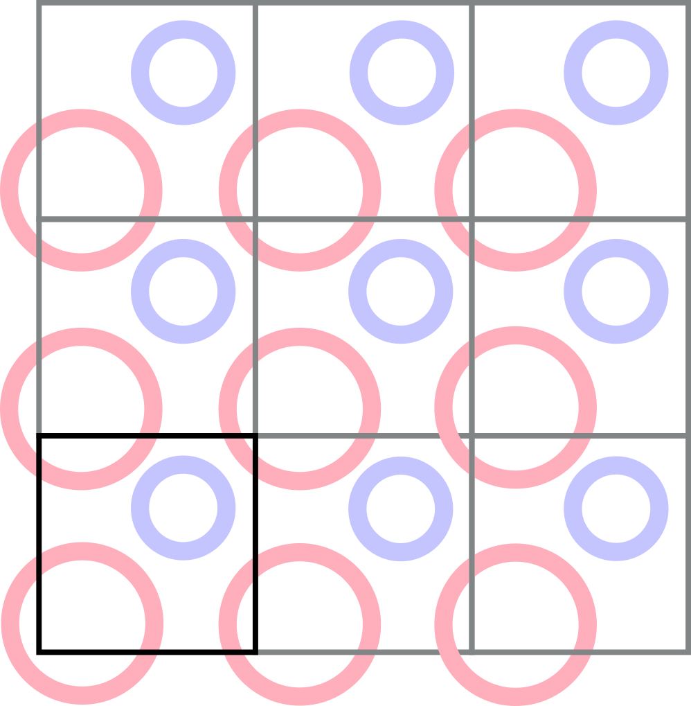
Let us consider a finite system (a molecule) that is composed of $N$ repeated cells, such as the one shown in the right. We assume that the energy in this system is given by a sum over atomic pairs of a function $g_{ij}(d_{ij})$ that depends only on the nature of the atoms and the distance between them, with $\begin{equation} g_{ij}(d_{ij}) = g_{ji}(d_{ji}) \end{equation}$. The $g_{ij}$ also has the property that it decays with distance quickly enough that an infinite sum over atomic pairs in three dimensions is absolutely convergent. For instance, if $g_{ij}$ represents a dispersion interaction, the leading term in the asymptotic limit would be $d_{ij}^{-6}$, which meets this convergence requirement.

The pairwise energy is calculated as:

$$\begin{equation} E = -\sum^{\rm all}_{i>j} g_{ij}(d_{ij}) \end{equation}$$

where the sum runs over all unique pairs of atoms in the whole system. Since $g_{ij} = g_{ji}$, we can write this more conveniently as:

$$\begin{equation} E = -\frac{1}{2}\sum^{\rm all}_{i\neq j} g_{ij}(d_{ij}) \end{equation}$$

This time we use a double sum over all atoms in the system, adding the equal ij and ji contributions and then dividing by two.

We now focus on a single atom and consider shells of other atoms around it. For a shell at a distance $d$, the number of atoms inside the shell is roughly proportional to its surface ($4\pi d^2$) and, since $g_{ij}(d_{ij})$ decays with distance faster than $d_{ij}^{-2}$, then the contribution from atomic shells at increasing distance from the central atom decays as well. Therefore, a given atom only perceives the interactions from a sphere of atoms up to a certain distance. This sphere of atoms is called the environment of the atom in the rest of this document.

If $N$ is large enough, then most of the atoms in the system see a full environment around them (the bulk atoms). The exception are the atoms on the edges and surface of the system. The energy contribution from the edge and surface atoms decreases relative to the bulk atoms as $N$ increases. This is because the number of atoms on the surface is proportional to $R^2$ and the number of atoms in the bulk increases as $R^3$, where $R$ is some length measure of the system size (e.g. its radius). Therefore, for large $N$, we can approximate the average energy per cell as:

$$\begin{equation} \frac{E}{N} \approx -\frac{1}{2}\sum_i^{\rm cell}\sum_j^{\rm all}{\vphantom{\sum}}^{\prime} g_{ij}(d_{ij}) \approx -\frac{1}{2}\sum_i^{\rm cell}\sum_j^{\rm env}{\vphantom{\sum}}^{\prime} g_{ij}(d_{ij}) \end{equation}$$

The prime means that the sum includes all atoms in the whole system or in the environment except for $i = j$. In the second sum, we replaced the sum over all atoms in the system with a sum over an environment that is the union of the environments of all atoms in the cell over which index i runs. In the limit of infinite $N$ (the thermodynamic limit) this expression becomes exact, and we write the pairwise energy per cell as:

$$\begin{equation} E_{\rm cell} = \lim_{N\to\infty} \frac{E}{N} = -\frac{1}{2}\sum_i^{\rm cell}\sum_j^{\rm env}{\vphantom{\sum}}^{\prime} g_{ij}(d_{ij}) \end{equation}$$

Because the system is periodic, we write this expression equivalently as a double sum over atoms in the unit cell plus a sum over lattice vectors:

$$\begin{equation} E_{\rm cell} = -\frac{1}{2}\sum_{ij}^{\rm cell}\sum_a{\vphantom{\sum}}^{\prime} g_{ij}(d^a_{ij}) \end{equation}$$

where $a$ runs over lattice vectors in the environment and the prime in the second equation indicates that the case where $i = j$ and $a = {\bf 0}$ is discarded. The distance with the lattice vector superscript is defined as:

$$\begin{equation} d_{ij} = \lvert {\bf x}_i - {\bf x}_j \rvert \quad ; \quad d^a_{ij} = \lvert {\bf x}_i - {\bf x}_j + {\bf R}_a \rvert \end{equation}$$

Note that $d_{ij} = d_{ji}$ but $d_{ij}^a = d_{ji}^{-a}$. We can always choose the environment in a way that if a lattice vector ${\bf R}_a$ is in the environment then its opposite $-{\bf R}_a$ is also included. With this assumption, we can use that $\begin{equation} g_{ij}(d_{ij}^a) = g_{ji}(d_{ji}^{-a}) \end{equation}$ to note that the double sum above contains terms that are twice repeated and re-write the energy as a sum over pairs of atoms in the unit cell:

$$\begin{equation} E_{\rm cell} = -\sum_{i\geq j}^{\rm cell}\sum_a{\vphantom{\sum}}^{\prime} g_{ij}(d^a_{ij}) \end{equation}$$

Distance Derivatives

The calculation of the derivatives of the energy with respect to the atomic positions requires the derivatives of the distance between two atoms. In the general case, the distance is:

$$\begin{equation} d^a_{ij} = \lvert {\bf x}_i - {\bf x}_j + {\bf R}_a \rvert \end{equation}$$

The first derivatives are:

$$\begin{align} \frac{\partial d_{ij}^a}{\partial x_{i\alpha}} & = \frac{({\bf x}_i - {\bf x}_j + {\bf R}_a)_\alpha}{d_{ij}^a} \\ \frac{\partial d_{ij}^a}{\partial x_{j\alpha}} & = \frac{({\bf x}_j - {\bf x}_i - {\bf R}_a)_\alpha}{d_{ij}^a} \end{align}$$

where $\alpha$ is the Cartesian coordinate (one of x, y, and z). Note that:

$$\begin{equation} \frac{\partial d_{ij}^a}{\partial x_{i\alpha}} = -\frac{\partial d_{ij}^a}{\partial x_{j\alpha}} \end{equation}$$

For the second derivatives, we have six possibilities resulting from the three combinations of the two indices (ii, jj, ij) and the two cases when $\alpha = \beta$ and $\alpha \neq \beta$. We start with the ii case:

$$\begin{align} \frac{\partial^2 d_{ij}^a}{\partial x_{i\alpha} \partial x_{i\alpha}} & = \frac{1}{d_{ij}^a} - \frac{({\bf x}_i - {\bf x}_j + {\bf R}_a)_\alpha^2}{(d_{ij}^a)^3} = - \frac{({\bf x}_{j\alpha} - {\bf x}_{i\alpha} - {\bf R}_{a\alpha} - d_{ij}^a) ({\bf x}_{j\alpha} - {\bf x}_{i\alpha} - {\bf R}_{a\alpha} + d_{ij}^a)}{(d_{ij}^a)^3} \\ \frac{\partial^2 d_{ij}^a}{\partial x_{i\alpha} \partial x_{i\beta}} & = -\frac{({\bf x}_i - {\bf x}_j + {\bf R}_a)_\alpha ({\bf x}_i - {\bf x}_j + {\bf R}_a)_\beta}{(d_{ij}^a)^3} \end{align}$$

Combining the two expressions:

$$\begin{equation} \frac{\partial^2 d_{ij}^a}{\partial x_{i\alpha} \partial x_{i\beta}} = \frac{\delta_{\alpha\beta}}{d_{ij}^a} -\frac{({\bf x}_i - {\bf x}_j + {\bf R}_a)_\alpha ({\bf x}_i - {\bf x}_j + {\bf R}_a)_\beta}{(d_{ij}^a)^3} \end{equation}$$

and the others can be obtained by using the index switch property of the first derivative:

$$\begin{align} \frac{\partial^2 d_{ij}^a}{\partial x_{i\alpha} \partial x_{j\alpha}} & = -\frac{\partial^2 d_{ij}^a}{\partial x_{i\alpha} \partial x_{i\alpha}} \\ \frac{\partial^2 d_{ij}^a}{\partial x_{j\alpha} \partial x_{j\alpha}} & = -\frac{\partial^2 d_{ij}^a}{\partial x_{i\alpha} \partial x_{j\alpha}} = \frac{\partial^2 d_{ij}^a}{\partial x_{i\alpha} \partial x_{i\alpha}} \\ \frac{\partial^2 d_{ij}^a}{\partial x_{i\alpha} \partial x_{j\beta}} & = -\frac{\partial^2 d_{ij}^a}{\partial x_{i\alpha} \partial x_{i\beta}} \\ \frac{\partial^2 d_{ij}^a}{\partial x_{j\alpha} \partial x_{j\beta}} & = -\frac{\partial^2 d_{ij}^a}{\partial x_{i\alpha} \partial x_{j\beta}} = \frac{\partial^2 d_{ij}^a}{\partial x_{i\alpha} \partial x_{i\beta}} \end{align}$$

In the most general case:

$$\begin{equation} \frac{\partial^2 d_{ij}^a}{\partial x_{i\alpha} \partial x_{j\beta}} = (-1)^{\delta_{ij}} \left[ \frac{({\bf x}_i - {\bf x}_j + {\bf R}_a)_\alpha ({\bf x}_i - {\bf x}_j + {\bf R}_a)_\beta}{(d_{ij}^a)^3} - \frac{\delta_{\alpha\beta}}{d_{ij}^a} \right] \end{equation}$$

The case where $j$ is an atom in the environment (instead of the cell) gives exactly the same derivatives, since it reduces to having $a = {\bf 0}$ in the expressions above.

Atomic Forces

The pairwise energy expression is (the “cell” subscript of the energy has been dropped for simplicity):

$$\begin{equation} E = -\sum_{i\geq j}^{\rm cell}\sum_a{\vphantom{\sum}}^{\prime} g_{ij}(d^a_{ij}) \end{equation}$$

The component $\alpha$ of the force exerted on atom i is defined as:

$$\begin{equation} F_{k\alpha} = -\frac{\partial E}{\partial x_{k\alpha}} \end{equation}$$

Of all the terms in the sum, only those involving atom $k$ will give a contribution. Since the sum runs over all pairs, these terms will either be $ik$, if $i \geq k$, or $ki$, if $i < k$. Hence:

$$\begin{equation} F_{k\alpha} = \frac{\partial}{\partial x_{k\alpha}} \left( \sum_{i\geq j}^{\rm cell}\sum_a{\vphantom{\sum}}^{\prime} g_{ij}(d^a_{ij})\right) = \sum_{i=1}^{k-1} \sum_a{\vphantom{\sum}}^{\prime} \frac{\partial g_{ki}(d^a_{ki})}{\partial x_{k\alpha}} +\sum_{i=k}^{\rm cell} \sum_a{\vphantom{\sum}}^{\prime} \frac{\partial g_{ik}(d^a_{ik})}{\partial x_{k\alpha}} \end{equation}$$

Note that:

$$\begin{equation} g_{ik}(d_{ik}^a) = g_{ki}(d_{ik}^a) = g_{ki}(d_{ki}^{-a}) \end{equation}$$

The sum over the environment lattice vectors contains all $a$ and $-a$ pairs, which means:

$$\begin{equation} \sum_a{\vphantom{\sum}}^{\prime} g_{ik}(d_{ik}^{a}) = \sum_a{\vphantom{\sum}}^{\prime} g_{ki}(d_{ki}^{-a}) = \sum_a{\vphantom{\sum}}^{\prime} g_{ki}(d_{ki}^{a}) \end{equation}$$

Therefore, we can combine the two partial sums into one and then apply the chain rule:

$$\begin{equation} F_{k\alpha} = \sum_{i=1}^{\rm cell} \sum_a{\vphantom{\sum}}^{\prime} \frac{\partial g_{ki}(d^a_{ki})}{\partial x_{k\alpha}} = \sum_{i=1}^{\rm cell} \sum_a{\vphantom{\sum}}^{\prime} g_{ki}^{\prime}(d^a_{ki}) \frac{\partial d_{ki}^a}{\partial x_{k\alpha}} \end{equation}$$

where $g^\prime(d)$ is the distance derivative of the $g(d)$ function. Unpacking the distance derivative, we arrive at the expression for the atomic force:

$$\begin{equation} F_{k\alpha} = \sum_{i=1}^{\rm cell} \sum_a{\vphantom{\sum}}^{\prime} g_{ki}^{\prime}(d^a_{ki}) \frac{({\bf x}_k - {\bf x}_i - {\bf R}_a)_\alpha}{d_{ki}^a} = \sum_{i=1}^{\rm cell} \sum_a{\vphantom{\sum}}^{\prime} g_{ik}^{\prime}(d^a_{ik}) \frac{({\bf x}_k - {\bf x}_i - {\bf R}_a)_\alpha}{d_{ik}^a} \end{equation}$$

Stress and Strain

To calculate the strain tensor, we consider an infinitesimal uniform deformation of the solid given by the strain tensor $\bf \varepsilon$. The positions of the atoms in the deformed geometry are given by:

$$\begin{equation} {\bf x}^\prime = {\bf x} ({\bf 1} + {\bf \varepsilon}) \end{equation}$$

The strain tensor is symmetric ($\varepsilon_{\alpha\beta} = \varepsilon_{\beta\alpha}$) because we are not interested in whole-body rotations of the solid. The stress tensor is defined as:

$$\begin{equation} \sigma_{\alpha\beta} = \frac{1}{V}\frac{\partial E}{\partial \varepsilon_{\alpha\beta}} \end{equation}$$

with $V$ the unit cell volume.

As in the case of the forces, we first calculate the distance derivatives with respect to the strain, then apply the chain rule. The interatomic distance between atoms i and j separated by lattice vector $a$ is given by:

$$\begin{equation} (d_{ij}^a)^2 = ({\bf x}_i - {\bf x}_j + {\bf R}_a) \cdot ({\bf x}_i - {\bf x}_j + {\bf R}_a)^T \end{equation}$$

When the strain is applied, the distance becomes:

$$\begin{equation} (d_{ij}^{a})^2 = ({\bf x}_i - {\bf x}_j + {\bf R}_a) ({\bf 1} + {\bf \varepsilon})({\bf 1} + {\bf \varepsilon})^T ({\bf x}_i - {\bf x}_j + {\bf R}_a)^T \end{equation}$$

Because the strain is infinitesimal, we can neglect any term that contains a product of two strains. Therefore, the strain matrix product in the middle of this expression simplifies to:

$$\begin{equation} ({\bf 1} + {\bf \varepsilon})({\bf 1} + {\bf \varepsilon})^T = {\bf 1} + {\bf \varepsilon} + {\bf \varepsilon}^T + {\bf \varepsilon}{\bf \varepsilon}^T \approx {\bf 1} + 2 {\bf \varepsilon} \end{equation}$$

where we used the fact that $\varepsilon = \varepsilon^T$. This transformation simplifies the distance expression:

$$\begin{equation} (d_{ij}^{a})^2 = \sum_{\alpha\beta} (x_{i\alpha} - x_{j\alpha} + R_{a\alpha}) (\delta_{\alpha\beta} + 2\varepsilon_{\alpha\beta}) (x_{i\beta} - x_{j\beta} + R_{a\beta}) \end{equation}$$

Taking the derivative with respect to an element of the strain tensor:

$$\begin{equation} 2 d_{ij}^{a} \frac{\partial d_{ij}^{a}}{\partial \varepsilon_{\alpha\beta}} = 2 (x_{i\alpha} - x_{j\alpha} + R_{a\alpha}) (x_{i\beta} - x_{j\beta} + R_{a\beta}) \end{equation}$$

and solving, we have:

$$\begin{equation} \frac{\partial d_{ij}^{a}}{\partial \varepsilon_{\alpha\beta}} = \frac{(x_{i\alpha} - x_{j\alpha} + R_{a\alpha}) (x_{i\beta} - x_{j\beta} + R_{a\beta})}{d_{ij}^{a}} \end{equation}$$

From this, the stress tensor is obtained by straightforward application of the chain rule:

$$\begin{equation} E = -\frac{1}{2}\sum_{ij}^{\rm cell}\sum_a{\vphantom{\sum}}^{\prime} g_{ij}(d^a_{ij}) \end{equation}$$ $$\begin{align} \sigma_{\alpha\beta} & = \frac{1}{V}\frac{\partial E}{\partial \varepsilon_{\alpha\beta}} = -\frac{1}{2V}\sum_{ij}^{\rm cell}\sum_a{\vphantom{\sum}}^{\prime} g^{\prime}_{ij}(d^a_{ij}) \frac{\partial d^a_{ij}}{\partial \varepsilon_{\alpha\beta}} \\ & = -\frac{1}{2V}\sum_{ij}^{\rm cell}\sum_a{\vphantom{\sum}}^{\prime} g^{\prime}_{ij}(d^a_{ij}) \frac{({\bf x}_{i} - {\bf x}_{j} + {\bf R}_{a})_\alpha ({\bf x}_{i} - {\bf x}_{j} + {\bf R}_{a})_\beta}{d_{ij}^{a}} \end{align}$$

The Dynamical Matrix

Phonon eigenvectors and phonon frequencies are calculated by diagonalizing the dynamical matrix:

$$\begin{equation} \sum_{i\alpha} D_{i\alpha}^{j\beta}({\bf q}) \varepsilon_n^{i\alpha}({\bf q}) = \omega_{n,{\bf q}}^2\varepsilon_n^{j\beta}({\bf q}) \end{equation}$$

where ${\bf \varepsilon}_n({\bf q})$ is the nth phonon eigenvector at vector $\bf q$ in the first Brillouin zone. The phonon eigenvectors have $3n$ elements and the dynamical matrix is a $3n\times 3n$ Hermitian matrix that is defined as:

$$\begin{equation} D_{i\alpha}^{j\beta}({\bf q}) = \frac{1}{\sqrt{M_iM_j}} C_{i\alpha}^{j\beta}({\bf q}) \end{equation}$$

where the $\bf C$ matrix is:

$$\begin{equation} C_{i\alpha}^{j\beta}({\bf q}) = \sum_a \Phi_{i\alpha}^{j\beta a} e^{i{\bf q}\cdot {\bf R}_a} \end{equation}$$

The $\bf \Phi$ matrix, which is the Fourier transform of $\bf C$, is called the interatomic force constant matrix (IFC). It is defined as:

$$\begin{equation} \Phi_{i\alpha}^{j\beta a} = \frac{\partial^2 E}{\partial x^0_{i\alpha} \partial x_{j\beta}^a} \end{equation}$$

The IFC matrix is calculated as the second derivative of the energy with respect to atomic displacements (equivalently, positions). One of the atoms (i) is in the unit cell, and the other (j) is translated by a lattice vector $a$. Note that, because of translational symmetry:

$$\begin{equation} \frac{\partial^2 E}{\partial x^a_{i\alpha} \partial x_{j\beta}^b} = \frac{\partial^2 E}{\partial x^0_{i\alpha} \partial x_{j\beta}^{b-a}} \end{equation}$$

it does not make much sense to have more than one lattice vector indexing the IFC matrix. Using the definition of atomic force, we have:

$$\begin{equation} \Phi_{i\alpha}^{j\beta a} = \frac{\partial E}{\partial x^0_{i\alpha} \partial x_{j\beta}^a} = - \frac{\partial F_{i\alpha}}{\partial x_{j\beta}^a} \end{equation}$$

The atomic force is:

$$\begin{equation} F_{i\alpha} = \sum_{j=1}^{\rm env} g_{ij}^{\prime}(d^a_{ij}) \frac{({\bf x}_i - {\bf x}^a_j)_\alpha}{d_{ij}^a} \end{equation}$$

where in this case we sum over the environment directly instead of using a sum over lattice vectors. We have added an $a$ superscript to environment atom j to keep track of which lattice vector it corresponds to.

Let us first consider the case in which atom $i$ and atom $j$ translated by $a$ are different. In this case, only one of the terms in the atomic force sum will contribute to the IFC matrix element $\Phi_{i\alpha}^{j\beta a}$, namely, the one whose index corresponds to atom j translated by lattice vector $a$. We define the distance function $h(d)$ as:

$$\begin{equation} h_{ij}(d) = \frac{g^{\prime}_{ij}(d)}{d} \end{equation}$$

so the IFC matrix can be written as:

$$\begin{equation} \Phi_{i\alpha}^{j\beta a} = - \frac{\partial F_{i\alpha}}{\partial x_{j\beta}^a} = - \frac{\partial}{\partial x_{j\beta}^a} \left( h_{ij}(d_{ij}^a) ({\bf x}_i - {\bf x}_j^a)_\alpha \right) \end{equation}$$

with ${\bf x}_j^a = {\bf x}_j + {\bf R}_a$. If $\alpha \neq \beta$,

$$\begin{equation} \Phi_{i\alpha}^{j\beta a} = h_{ij}^{\prime}(d_{ij}^a) \frac{({\bf x}_i - {\bf x}_j^a)_\alpha ({\bf x}_i - {\bf x}_j^a)_\beta}{d_{ij}^a} \end{equation}$$

and if $\alpha = \beta$,

$$\begin{equation} \Phi_{i\alpha}^{j\beta a} = h_{ij}^{\prime}(d_{ij}^a) \frac{({\bf x}_i - {\bf x}_j^a)^2_\alpha}{d_{ij}^a} + h_{ij}(d_{ij}^a) \end{equation}$$

Combining the two results, we have:

$$\begin{equation} \Phi_{i\alpha}^{j\beta a} = h_{ij}^{\prime}(d_{ij}^a) \frac{({\bf x}_i - {\bf x}_j^a)_\alpha ({\bf x}_i - {\bf x}_j^a)_\beta}{d_{ij}^a} + \delta_{\alpha\beta} h_{ij}(d_{ij}^a) \end{equation}$$

In the case where $i = j$ and $a = {\bf 0}$, we have:

$$\begin{align} \Phi_{i\alpha}^{i\beta 0} & = -\frac{\partial F_{i\alpha}}{\partial x_{i\beta}} = - \sum_j^{\rm env} \left( h_{ij}^\prime(d_{ij}^a) \frac{({\bf x}_i - {\bf x}_j)_\alpha ({\bf x}_i - {\bf x}_j)_\beta} {d_{ij}^a} + \delta_{\alpha\beta} h_{ij}(d_{ij}^a) \right) \\ & = - \sum_j^{\rm cell} \sum_{a}{\vphantom{\sum}}^{\prime} \Phi_{i\alpha}^{j\beta a} \end{align}$$

Therefore, the same-atom IFC matrix elements can be calculated using the zero-sum rule:

$$\begin{equation} \sum_j^{\rm cell} \sum_a \Phi_{i\alpha}^{j\beta a} = 0 \quad {\rm for\ all}\quad i,\alpha,\beta \end{equation}$$

Finally, the massless dynamical matrix is:

$$\begin{align} C_{i\alpha}^{j\beta}({\bf q}) & = \sum_a \Phi_{i\alpha}^{j\beta a} e^{i{\bf q}\cdot {\bf R}_a} = \Phi_{i\alpha}^{j\beta 0} + \sum_{a \neq 0} \Phi_{i\alpha}^{j\beta a} e^{i{\bf q}\cdot {\bf R}_a} \\ & = -\sum_k^{\rm cell} \sum_a{\vphantom{\sum}}^{\prime} \Phi_{i\alpha}^{k\beta a} + \sum_{a\neq 0} \Phi_{i\alpha}^{j\beta a} e^{i{\bf q}\cdot {\bf R}_a} \end{align}$$

with:

$$\begin{equation} \Phi_{i\alpha}^{j\beta a} = h_{ij}^{\prime}(d_{ij}^a) \frac{({\bf x}_i - {\bf x}_j^a)_\alpha ({\bf x}_i - {\bf x}_j^a)_\beta}{d_{ij}^a} + \delta_{\alpha\beta} h_{ij}(d_{ij}^a) \end{equation}$$

Pairwise Energy Functions

The expressions above allow the calculation of forces, stress, and dynamical matrix contributions from any pairwise atomic energy term. For a pairwise interaction given by:

$$\begin{equation} E = -\sum^{\rm all}_{i>j} g_{ij}(d_{ij}) \end{equation}$$

we only need the $g_{ij}(d)$ function, its derivative ($g_{ij}^{\prime}(d)$), the $h_{ij}(d) = g_{ij}^{\prime}(d) / d$ function, and its derivative ($h_{ij}^{\prime}(d)$). These are easily obtained from a computer algebra program such as maxima (see at the end for the cantor script). The radial functions for the D2 and XDM dispersion corrections are given now.

Pairwise Energy Functions for the D2 Dispersion Correction

We first define the exponential function:

$$\begin{equation} e_{ij}(d) = \exp\left[ -\beta\left(\frac{d}{R_{ij}} - 1\right)\right] \end{equation}$$

The pairwise energy:

$$\begin{equation} g_{ij}(d) = \frac{C_6^{ij} s_6}{d^6 (1 + e_{ij}(d))} \end{equation}$$

where $s_6 = 0.75$ and $\beta = 20$ are adjustable parameters, $C_6^{ij}$ are the (fixed) dispersion coefficients and $R_{ij}$ is the sum of van der Waals radii. The distance derivative of this function is:

$$\begin{equation} g_{ij}^{\prime}(d) = g_{ij}(d) \left(\frac{\beta e_{ij}(d)}{R_{ij} (1+e_{ij}(d))} - \frac{6}{d}\right) \end{equation}$$

The h-function is:

$$\begin{equation} h_{ij}(d) = \frac{g_{ij}^{\prime}(d)}{d} = \frac{g_{ij}(d)}{d} \left(\frac{\beta e_{ij}(d)}{R_{ij} (1+e_{ij}(d))} - \frac{6}{d}\right) \end{equation}$$

and its derivative is:

$$\begin{equation} h^{\prime}_{ij}(d) = \frac{g_{ij}(d)}{d} \left( \frac{48}{d^2} - \frac{13 \beta e_{ij}(d)}{R_{ij} d (1+e_{ij}(d))} - \frac{\beta^2 e_{ij}(d)}{R_{ij}^2} \frac{1-e_{ij}(d)}{(1 + e_{ij}(d))^2}\right) \end{equation}$$

Pairwise Energy Functions for the XDM Dispersion Correction

The XDM dispersion coefficients depend on the geometry of the system but they usually change very slowly when atoms move and, in general, it is a good approximation to assume that the dispersion coefficients are constant. The pairwise energy contribution for each pair is:

$$\begin{equation} g_{ij}(d) = \frac{C_6^{ij}}{R_{ij}^6 + d^6} + \frac{C_8^{ij}}{R_{ij}^8 + d^8} + \frac{C_{10}^{ij}}{R_{ij}^{10} + d^{10}} \end{equation}$$

and its derivative:

$$\begin{equation} g_{ij}^{\prime}(d) = -\frac{6C_6^{ij}d^5}{(R_{ij}^6 + d^6)^2} - \frac{8C_8^{ij}d^7}{(R_{ij}^8 + d^8)^2} - \frac{10C_{10}^{ij}d^9}{(R_{ij}^{10} + d^{10})^2} \end{equation}$$

The h-function is:

$$\begin{equation} h_{ij}(d) = \frac{g_{ij}^{\prime}(d)}{d} = -\frac{6C_6^{ij}d^4}{(R_{ij}^6 + d^6)^2} - \frac{8C_8^{ij}d^6}{(R_{ij}^8 + d^8)^2} - \frac{10C_{10}^{ij}d^8}{(R_{ij}^{10} + d^{10})^2} \end{equation}$$

and its derivative:

$$\begin{align} h^{\prime}_{ij}(d) & = -\frac{80 C_{10}^{ij} d^7}{(d^{10} + R_{ij}^{10})^2} + \frac{200 C_{10}^{ij} d^{17}}{(d^{10} + R_{ij}^{10})^3} - \frac{48 C_8^{ij} d^5}{(d^{8} + R_{ij}^{8})^2} \\ & + \frac{128 C_8^{ij} d^{13}}{(d^{8} + R_{ij}^{8})^3} - \frac{24 C_6^{ij} d^3}{(d^{6} + R_{ij}^{6})^2} + \frac{72 C_6^{ij} d^9}{(d^{6} + R_{ij}^{6})^3} \end{align}$$

Testing routines

A simple way to check the consistency of the four functions ($g$, $g^\prime$, $h$, $h^\prime$) is to use a small Fortran program that writes a table of values in a simple case (e.g. graphite), then use octave to verify all the values against numerical derivatives of $g$ and $h$. An advantage of this method is that, once written and tested, the routines can be transported as a whole into Quantum ESPRESSO. For D2:

subroutine calcgh_d2(d,g,gp,h,hp)
  implicit none
  real*8, intent(in) :: d
  real*8, intent(out) :: g, gp, h, hp

  real*8 :: ed, fij, d6, d7, d2, scal6, c6_ij, r_sum, beta

  ! graphite
  scal6 = 0.75d0
  c6_ij = 60.71d0
  r_sum = 5.488d0
  beta = 20d0

  d2 = d * d
  d6 = d**6
  d7 = d6 * d
  ed = exp(-beta * (d / r_sum - 1.d0))
  fij = 1.d0 / (1.d0 + ed)
  g = c6_ij * scal6 / d6 * fij
  gp = c6_ij * scal6 / d6 / (1.d0 + ed) * (beta * ed / r_sum / (1.d0 + ed) - 6.d0 / d)
  h = gp / d
  hp = c6_ij * scal6 / d7 / (1.d0 + ed) * (48.d0 / d2 - &
     13.d0 * beta * ed / r_sum / d / (1.d0 + ed) - &
     beta**2 * ed / r_sum**2 / (1.d0 + ed)**2 * (1.d0 - ed))

end subroutine calcgh_d2

For XDM:

subroutine calcgh_xdm(d,g,gp,h,hp)
  implicit none
  real*8, intent(in) :: d
  real*8, intent(out) :: g, gp, h, hp

  real*8 :: c6, c8, c10, rvdw
  real*8 :: d2, d4, d6, d8, d10, dpr6, dpr8, dpr10, r2, r6, r8, r10
  real*8 :: d5, d7, d9, dpr6sq, dpr8sq, dpr10sq, d17, d13, d3, dpr6cub
  real*8 :: dpr8cub, dpr10cub

  ! graphite
  c6 = 1.771066d+01 * 2d0 ! to ry
  c8 = 6.829096d+02 * 2d0 ! to ry
  c10 = 2.876529d+04 * 2d0 ! to ry
  rvdw = 7.308851d0

  r2 = rvdw * rvdw
  r6 = r2 * r2 * r2
  r8 = r6 * r2
  r10 = r8 * r2

  d2 = d * d
  d3 = d2 * d
  d4 = d2 * d2
  d5 = d4 * d
  d6 = d4 * d2
  d7 = d6 * d
  d8 = d6 * d2
  d9 = d8 * d
  d10 = d8 * d2
  d13 = d6 * d7
  d17 = d10 * d7

  dpr6 = r6 + d6
  dpr8 = r8 + d8
  dpr10 = r10 + d10
  dpr6sq = dpr6 * dpr6
  dpr8sq = dpr8 * dpr8
  dpr10sq = dpr10 * dpr10
  dpr6cub = dpr6sq * dpr6
  dpr8cub = dpr8sq * dpr8
  dpr10cub = dpr10sq * dpr10

  g = c6 / dpr6 + c8 / dpr8 + c10 / dpr10
  gp = -10d0 * c10 * d9 / dpr10sq - 8d0 * c8 * d7 / dpr8sq - 6d0 * c6 * d5 / dpr6sq
  h = gp / d
  hp = -80d0 * c10 * d7 / dpr10sq + 200d0 * c10 * d17 / dpr10cub - 48d0 * c8 * d5 / dpr8sq &
     + 128d0 * c8 * d13 / dpr8cub - 24 * c6 * d3 / dpr6sq + 72d0 * c6 * d9 / dpr6cub

end subroutine calcgh_xdm

The octave script to verify the consistency of the implemented pairwise energy functions is:

load aa

d = aa(:,2);
g = aa(:,3);
gp = aa(:,4);
h = aa(:,5);
hp = aa(:,6);

gavg = 0.5 * (g(1:end-1)+g(2:end));
gpavg = 0.5 * (gp(1:end-1)+gp(2:end));
numgpavg = diff(g) ./ diff(d);
havg = 0.5 * (h(1:end-1)+h(2:end));
hpavg = 0.5 * (hp(1:end-1)+hp(2:end));
numhpavg = diff(h) ./ diff(d);

printf("gp = dg/dd (rel) : %.4e\n",max(abs(gpavg - numgpavg) ./ abs(gpavg)));
printf("h = gp/d   (abs) : %.4e\n",max(abs(h - gp ./ d)));
printf("hp = dh/dd (rel) : %.4e\n",max(abs(hpavg - numhpavg) ./ abs(hpavg)));

The output of this test for XDM is:

gp = dg/dd (rel) : 1.1023e-04
h = gp/d   (abs) : 1.3031e-17
hp = dh/dd (rel) : 4.5022e-04

indicating that the numerical and analytical derivatives agree with each other to about one in ten thousand. The program and script files are given at the end of this document.

The consistency of the $g(d)$ routine can be tested in Quantum ESPRESSO directly by performing the dispersion energy sum from within the phonon calculation. The dispersion energy in ph.x and the one obtained from pw.x must be equal.

Supporting files

Program and script for testing the pairwise energy routines:

• check-calcgh.tar.xz

Cantor notebook file with the derivatives of the pairwise energy functions:

• distance.cws

QE implementation of the XDM dynamical matrix contribution:

• d2ionq_xdm.f90

QE implementation of the D2 dynamical matrix contribution:

• d2ionq_mm.f90