Integration of Atomic Properties with Grids
Bader Volumes and Charges
In this example, we examine how to compute Bader atomic properties, specifically charges and volumes, in periodic solids using different electronic structure software using the plane-waves/pseudopotentials approach. For the integration, we use the Yu-Trinkle method (YT keyword) but the same can be done with Henkelman et al.’s method (BADER keyword).
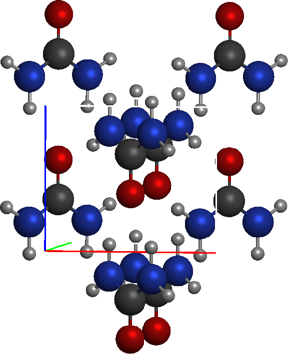
For illustration, we use the urea crystal. When it crystallizes, urea forms an orthorhombic molecular crystal with 16 atoms in the unit cell (2 molecules), shown on the right. There are chains of double hydrogen bonds all along the c axis, and all molecules in the crystal are equivalent by symmetry.
The input files necessary for this example can be generated from critic2’s internal library of structures. For instance, to create a Quantum ESPRESSO input, we do:
crystal library urea
write urea.scf.in
This generates an input file template. The particular keywords this template has are most likely not what you want, but the structure, which is after all the difficult part to write, is correct. Likewise, we can generate inputs for VASP or abinit with:
crystal library urea
write POSCAR
write urea.abin
Output formats for many other programs are supported as well.
Quantum ESPRESSO
How it Works
Quantum ESPRESSO does DFT
calculations in periodic solids using plane waves. A typical
calculation of the atomic charges has two steps. In the first step,
you carry out the SCF calculation with the pw.x program on a
.scf.in input file, such as the one generated in the example
above. This generates the converged wavefunction, which is stored in
QE’s internal format.
To extract the densities you use the pp.x (post-process) program to
ask QE to write the density on a three-dimensional grid. (In a
plane-waves code the density and wavefunctions are expressed naturally
as uniform three-dimensional grids.) pp.x generates two types of
file formats for the 3D density grid: Gaussian cube files (.cube)
and xcrysden’s .xsf files. We will use the former, but critic2 can
also understand and use .xsf files. Note that both cube and xsf
files contain also the structural information, so you can use them to
read the crystal structure into critic2 as well as the density at any
time.
There are several ways of calculating the atomic charges, depending on the type of pseudopotential you use. Plane-wave/pseudopotentials codes use pseudopotentials for two reasons: 1) remove the core electrons and 2) smooth out the system’s wavefunctions close to the atoms, in order to prevent having to use an extremely large number of plane waves to represent the oscillations close to the atomic nuclei. Because of this the density peaks close to the nuclei are not as high as they should be and, in systems with significant charge transfer, the maxima at the nuclei may be missing altogether. Therefore, the electron smoothed density used in QE (the pseudo-density) cannot be used to calculate the QTAIM atomic basins, and we must have a way to recover the all-electron density from the calculation. Depending on the method and pseudopotential employed, this may be easy or hard.
Ideally, you want to use the PAW method because the information about
the conversion to the all-electron wavefunctions is not lost, and
therefore you keep the option of reconstructing the all-electron
density. In recent versions of QE, this option is given by the
plot_num=21 option in pp.x. Here is an example input for pp.x
that writes the reconstructed all-electron density to a cube file
(rhoae.cube):
&inputpp
 prefix='urea',
 outdir='.',
 plot_num=21,
/
&plot
 iflag=3,
 output_format=6,
 fileout='rhoae.cube',
/
If your version of QE is not very recent, then plot_num=21 may not
be available to you. In that case, you can still get the all-electron
valence density with plot_num=17, and then augment this density
with the core contribution calculated using critic2’s internal density
tables (see below).
The all-electron density is too steep close to the nuclei to be
efficiently represented by a grid and, consequently, it does not sum
to the correct number of electrons. Therefore, even though it gives
the correct atomic basins, integrating the all-electron density to
obtain the atomic charges is a poor idea. Instead, we integrate the
pseudo-density, which is the density actually used in the SCF
calculation and it is normalized to the number of valence
electrons. To obtain the pseudo-density from pp.x, you use the same
input as above but with plot_num=0. In the case of a non-PAW
calculation, using either norm-conserving or ultrasoft
pseudopotentials, plot_num=0 will be the only option available to
you and, in that case, the pseudo-density is used to calculate the
shape of the atomic basins as well. Although not ideal, experience has
shown that the calculated atomic charges are about the same as with
the correct all-electron density, provided core augmentation is
utilized.
To summarize, to calculate atomic volumes and charges you do:
PAW Calculation
If you ran a PAW calculation, get the all-electron density
(plot_num=21, rhoae.cube) and the pseudo-density (plot_num=0,
rho.cube) and integrate the latter in the basins of the former
with:
crystal rhoae.cube
load rhoae.cube
load rho.cube
integrable 2
yt
The basins are given by the reference field (rhoae.cube, the first
field loaded) and we define the second field (rho.cube) as the
integrand. The YT keyword launches the calculation of atomic
properties. This is the preferred option.
PAW Calculation (Old QE Version)
If you ran a PAW calculation but your QE version is old and you do
not have plot_num=21, then write the reconstructed valence density
(plot_num=17, rhoval.cube) and the pseudo-density (plot_num=0,
rho.cube) and integrate the latter in the basins of the former,
but using core augmentation to account for the missing core
electrons:
crystal rhoval.cube
load rhoval.cube zpsp c 4 o 6 n 5 h 1
load rho.cube
integrable 2
yt
Core augmentation is activated with the ZPSP option to LOAD, and we
need to give to critic2 the pseudopotential charges for each
atom. This value is equal to the atomic number minus the number of
core electrons removed in the calculation. In QE, this value can be
obtained by summing the numbers in the occ column under Valence
configuration in the corresponding .UPF file. The core
contribution for the given number of core electrons is added by
critic2 every time the field is evaluated using critic2’s internal
density tables.
NC or US Pseudopotential Calculation
If you ran a US or NC pseudopotential calculation, then you only
have the pseudodensity (plot_num=0, rho.cube). In this case,
load the pseudo-density twice and activate core augmentation the
first time. Use the core-augmented field to generate the atomic
basins and the non-augmented field as the integrand:
crystal rho.cube
load rho.cube zpsp c 4 o 6 n 5 h 1
load rho.cube
integrable 2
yt
VASP
To calculate Bader charges in VASP, you need to run the SCF
calculation in the usual way, but including the following tag in the
INCAR file:
LAECHG = .TRUE.
This will generate two additional files: the AECCAR0, containing the
core density, and the AECCAR2, containing the reconstructed valence
density. The sum of the two needs to be used to generate the atomic
basins, while the pseudo-density, contained in the CHGCAR file, is
integrated in them.
These operations can be all done within critic2 cheaply and without generating any additional files using the following input:
crystal CHGCAR
load AECCAR0
load AECCAR2
load as "$1+$2"
reference 3
load CHGCAR
integrable 4
yt
As with the cube files, any of the CHGCAR, AECCAR0, etc. files
specifies the crystal structure inside, so you can have it critic2
read it from any of them. (You can also use the POSCAR and the
POTCAR.) We load the AECCAR0 as field 1, and the AECCAR2 as
field 2, and create field 3 as the sum of those two files. Field 3 now
contains the all-electron density, and we set it as reference in order
to have it generate the atomic basins. Finally, we load the CHGCAR
file as field 4 and mark it as an integrand for our YT calculation.
Important note: occasionally, strange results may be obtained from
the integration of atomic charges with VASP due to noise in the
AECCAR0 file. To prevent this, do not use ADDGRID=.TRUE. in your
INCAR file.
Abinit
If you are using PAW datasets, then the reconstructed valence density can be obtained in abinit using:
prtden 2
in the input file. This creates two density files: the pseudo-density
(with suffix _DEN) and the reconstructed valence density
(_PAWDEN). Currently, there is no easy way to obtain the
all-electron density from abinit directly. In the case of a non-PAW
calculation, using either norm-conserving or ultrasoft
pseudopotentials, then prtden 2 is not available and you have to
use:
prtden 1
which writes the _DEN file only.
If you have the _PAWDEN file, the calculation of the atomic charges
is straightforward:
crystal urea_o_DEN
load urea_o_PAWDEN zpsp h 1 c 4 n 5 o 6
load urea_o_DEN
integrable 2
yt
The _DEN and _PAWDEN files both contain the structural information
about the crystal, so they can be used to read the crystal structure
in critic2 through the CRYSTAL keyword. The _PAWDEN density is
loaded as field 1 and is augmented with core electrons corresponding
to the pseudopotential charges (atomic number minus number of replaced
core electrons). The all-electron density obtained in this way is used
to generate the atomic basins. The pseudo-density (_DEN) is then
loaded as the second field and integrated inside the basins.
If you ran a non-PAW calculation, then replace the _PAWDEN file with
the _DEN file in the input above.
Output for Urea
The outputs from all the calculations above are very similar. The main table containing the results of the integration appears right at the end of the output:
* Integrated atomic properties
# (See key above for interpretation of column headings.)
# Integrable properties 1 to 4
# Id   cp   ncp   Name  Z   mult     Volume            Pop             Lap             $2
  1    1    1      C_   6   --   3.22216552E+01  4.21263334E+00  1.02937536E-01  2.19098664E+00
  2    2    1      C_   6   --   3.22216552E+01  4.21263334E+00  1.02937536E-01  2.19098664E+00
  3    3    2      H_   1   --   2.00349124E+01  5.13744359E-01 -3.64792425E-04  5.13705108E-01
  4    4    2      H_   1   --   2.00349124E+01  5.13744359E-01 -3.64792425E-04  5.13705108E-01
  5    5    2      H_   1   --   2.00349124E+01  5.13744359E-01 -3.64792425E-04  5.13705108E-01
  6    6    2      H_   1   --   2.00349124E+01  5.13744359E-01 -3.64792425E-04  5.13705108E-01
  7    7    3      H_   1   --   2.05322160E+01  5.11380307E-01 -1.96443849E-02  5.11335066E-01
  8    8    3      H_   1   --   2.05322160E+01  5.11380307E-01 -1.96443849E-02  5.11335066E-01
  9    9    3      H_   1   --   2.05322160E+01  5.11380307E-01 -1.96443849E-02  5.11335066E-01
  10   10   3      H_   1   --   2.05322160E+01  5.11380307E-01 -1.96443849E-02  5.11335066E-01
  11   11   4      O_   8   --   1.18754676E+02  9.40395235E+00 -1.26560690E-01  7.23176246E+00
  12   12   4      O_   8   --   1.18754676E+02  9.40395235E+00 -1.26560690E-01  7.23176246E+00
  13   13   5      N_   7   --   1.26002600E+02  8.28697652E+00  3.18207545E-02  6.26367524E+00
  14   14   5      N_   7   --   1.26002600E+02  8.28697652E+00  3.18207545E-02  6.26367524E+00
  15   15   5      N_   7   --   1.26002600E+02  8.28697652E+00  3.18207545E-02  6.26367524E+00
  16   16   5      N_   7   --   1.26002600E+02  8.28697652E+00  3.18207545E-02  6.26367524E+00
------------------------------------------------------------------------------------------------
  Sum                            9.68231575E+02  6.44815761E+01 -1.12894416E-12  4.80003598E+01
In this table, critic2 lists the 16 attractors it found, which in this
case are all associated to atoms in the system (there are no
non-nuclear maxima). It also gives the following columns: the
calculated atomic volumes (Volume), the all-electron density
integrated in its basins (Pop), the Laplacian of the all-electron
density (Lap), and the integral of field number 2 (the
pseudo-density) in the all-electron basins ($2). The last column
gives the valence electron population for each atom. The atomic charge
equals the pseudopotential charge minus the valence electron
population. For instance, the charge for carbon in this system would
be \(Z_{\rm psps} - N = 4 - 2.19 = 1.81\).
Because critic2 detects that urea is a molecular crystal, it will also helpfully list for you the integrated properties of the molecules as a whole:
* Integrated molecular properties
# (See key above for interpretation of column headings.)
# Integrable properties 1 to 4
# Mol     Volume            Pop             Lap             $2
  1     4.84115787E+02  3.22407881E+01 -1.12265058E-12  2.40001799E+01
  2     4.84115787E+02  3.22407881E+01 -6.32133235E-15  2.40001799E+01
The interpretation of the columns is the same, but this time the numbers refer to each of the two urea molecules in the unit cell. Because they are equivalent by symmetry, their volumes and electron populations are the same and the charge is zero (the sum of the pseudopotential charges in each molecule is 24).
- QE/PAW calculation (
qe_paw):## generate the pseudopotentials first ld1.x < h.in ld1.x < c.in ld1.x < n.in ld1.x < o.in ## run the SCF calculation pw.x < urea.scf.in > urea.scf.out ## get the densities pp.x < urea.rho.in > urea.rho.out pp.x < urea.rhoval.in > urea.rhoval.out pp.x < urea.rhoae.in > urea.rhoae.out ## run critic2 critic2 urea.cri urea.croIf the
rhoae.cubewas not generated, you are using an old version of QE. In that case, editurea.cri, comment out the first block and uncomment the second block. - QE/NC or US calculation (
qe_ncandqe_us):## generate the pseudopotentials first ld1.x < h.in ld1.x < c.in ld1.x < n.in ld1.x < o.in ## run the SCF calculation pw.x < urea.scf.in > urea.scf.out ## get the density pp.x < urea.rho.in > urea.rho.out ## run critic2 critic2 urea.cri urea.cro - VASP calculation: first, create the POTCAR file by concatenating the
POTCARs for C, H, O, and N, in that order. Then:
vasp critic2 urea.cri urea.cro - abinit:
abinit ## or abinis/abinip if you are running a really old version
critic2 urea.cri
Hirshfeld Integration
Hirshfeld Charges
Hirshfeld volumes and atomic charges can be calculated by grid integration using the HIRSHFELD keyword. The reference field must be a grid, and the integration is carried out on a grid with the same dimensions. For instance, for the urea example above calculated using QE and PAW, the Hirshfeld atomic properties can be obtained with:
crystal rho.cube
load rho.cube
hirshfeld
The result is very similar to the output of a Bader integrations:
* Integrated atomic properties
# Id   cp   ncp   Name  Z   mult     Volume            Pop             Lap
  1    1    1      C_   6   --   7.62964463E+01  3.82743786E+00  2.62543556E+00
[...]
  3    3    2      H_   1   --   4.72868033E+01  9.06486107E-01  9.22335042E-01
[...]
  11   11   4      O_   8   --   6.85164260E+01  6.22599870E+00 -2.51562267E+00
[...]
  13   13   5      N_   7   --   7.89839953E+01  5.16616905E+00 -1.85443836E+00
[...]
where “Pop” is the integral of the reference field and “Lap” the integral of its Laplacian. Since the reference field is the pseudo-density, “Pop” is the integrated Hirshfeld electron population in the corresponding atoms. In this calculation, the PAW datasets used for C, H, N, and O have 4, 1, 5, and 6 valence electrons respectively. Therefore, the Hirshfeld charges are: C = 6 - 3.827 = 2.173, H = 1 - 0.906 = 0.094, O = 6 - 6.226 = -0.226, and N = 5 - 5.166 = -0.166.
Hirshfeld Overlap Populations
Hirshfeld overlap populations can also be calculated with the HIRSHFELD keyword. If the scalar field integrated is an electron density, these quantities are related to the interatomic bond order. To get the overlap populations in the urea example, we need to add them as an integrable property using the INTEGRABLE keyword:
crystal rho.cube
load rho.cube
integrable 1 overlap
hirshfeld
The calculation takes longer than in the case of the charges and results in one table of overlap populations for every atom in the unit cell. Every row corresponds to the other atom in the pair, and the rows are sorted by distance to the reference atom:
# Atom 1 (cp=1, ncp=1, name=C, Z=6) at: 0.9999968  0.4999984  0.3274749
# Id   cp   ncp   Name  Z    Latt. vec.     ----  Cryst. coordinates ----       Distance        Overlap
  10   1    1      C    6    0   0   0   0.9999968    0.4999984    0.3274749    0.0000000    2.19178667
  149  11   4      O    8    0   0   0   0.9999968    0.4999984    0.6001924    2.4072660    0.52258093
  175  13   5      N    7    1   0   0   1.1470466    0.6470450    0.1776837    2.5479248    0.46667495
  196  15   5      N    7    0   0   0   0.8529469    0.3529485    0.1776837    2.5479453    0.46668283
[...]
  128  9    3      H    1    1   0  -2   1.8548290    0.3548306   -1.0403216   15.1074645    0.00000001
  97   7    3      H    1    1  -1  -2   1.1451645   -0.3548371   -1.0403216   15.1074846    0.00000001
  Total (Hirshfeld population).............................................................  3.82945379
The sum of the overlap populations equals the Hirshfeld population (number of electrons) for that atom.
Voronoi Deformation Density Charges
The deformation density is the electron density minus the promolecular density. The Voronoi deformation density (VDD) charges are calculated by integrating the deformation density in the Voronoi region of an atom, the set of points closer to that atom than to any other.
Atomic integrations in the Voronoi regions can be carried out using the VORONOI keyword. The Voronoi integrations are always done on grids, so the reference field must be a grid, and the integration is carried out on a grid of the same dimesions as the reference. Only smooth (slowly varying) scalar fields should be integrated on a grid; otherwise the numerical integration error will be too high.
Although the deformation density can be calculated using critic2’s
promolecular density (accesible with $0), it is better if the
program that generates the self-consistent density also writes a
promolecular density calculated with the same method. Two examples of
how to do this are given below: with Quantum ESPRESSO and with VASP.
Quantum ESPRESSO
For the urea example above, using Quantum ESPRESSO and PAW, the
deformation density can be written by using the plot_num=9 option in
pp.x. Assuming the resulting cube file is written to rhodef.cube,
the VDD charges can be calculated using:
crystal rhodef.cube
load rhodef.cube
voronoi
The output of Voronoi is similar to the Bader integration methods:
* Integrated atomic properties
# Id   cp   ncp   Name  Z   mult     Volume            Pop             Lap
  1    1    1      C_   6   --   4.63970561E+01 -1.78359676E-01  5.87903902E-01
[...]
  3    3    2      H_   1   --   8.37458327E+01 -1.32918872E-01 -8.45737309E-02
[...]
  11   11   4      O_   8   --   5.08817985E+01  3.33187749E-01 -6.18843287E-01
[...]
  13   13   5      N_   7   --   3.72016928E+01  1.87642259E-01  2.14109814E-01
[...]
--------------------------------------------------------------------------------
  Sum                            9.68231575E+02  1.87698750E-04 -1.15463195E-14
In this output, the “Pop” column is the reference field
(rhodef.cube) calculated in the Voronoi regions of each atom.
The VDD charges are minus this value, i.e.: C = 0.178,
H = 0.133, O = -0.332, N = -0.188. It is important to check the sum of
the VDD charges is zero, in the last row. This value is an
indicator of the numerical error incurred by the grid integration.
VASP
Using the LAECHG tag, it is possible to have VASP write the
reconstructed valence density (AECCAR2) and the valence promolecular
density (AECCAR1). (For the AECCAR1 to be written correctly,
ADDGRID must not be .TRUE..) To calculate the VDD charges, read
both files as scalar fields and then take the difference (promolecular
minus self-consistent):
crystal AECCAR1
load AECCAR1
load AECCAR2
load as "$1-$2"
Then set the newly created grid as reference and integrate it in the Voronoi regions.
reference 3
voronoi
The “Pop” column contains the VDD charges. As in the case of QE, it is important to check that the sum of the VDD charges is close to zero, to make sure the numerical error from the grid integration is not too high.
Example Files Package
Files: example_11_01.tar.xz.