Making STM plots with Quantum ESPRESSO and critic2

Obtaining the LDOS

Scanning tunneling microscopy (STM) is an experimental technique that maps the structure of a material by dragging a tip across its surface. A small bias voltage $V$ is applied to the tip such that electrons from the surface tunnel and create a current $I$ across the tip that is measured by the instrument. In the Tersoff-Hamann approximation, the current is proportional to the applied bias voltage and to the local density of states at the Fermi level, which is defined as:

$\begin{equation} \rho_{\rm loc}({\bf r},V) = \sum_{ {\bf k},n}^{E_F-eV\to E_F} |\psi_{ {\bf k},n}({\bf r})|^2 \end{equation}$

where the sum runs only over the one-electron states that have energies between $E_F-eV$ and $E_F$ . The LDOS corresponds to the electron density contributions from all states that are within $eV$ of the Fermi level. In Quantum ESPRESSO, a cube file containing this LDOS for the chosen bias voltage can be written using pp.x and option plot_num=5.

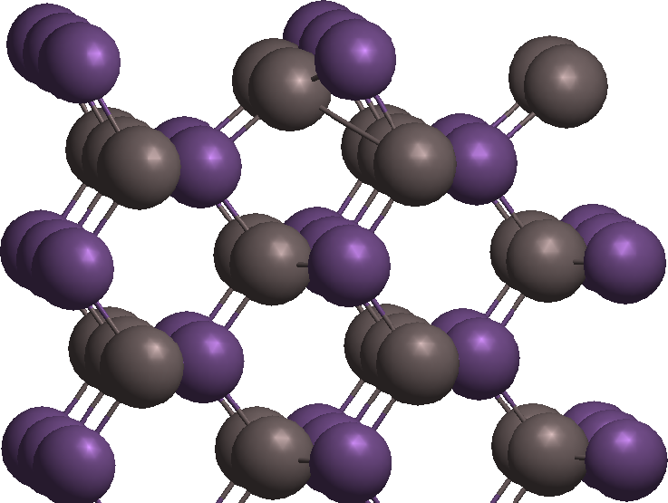
To illustrate how this works, we use the AlAs (110) surface provided in the Quantum ESPRESSO distribution (in the examples of the PP package, example03). The surface is shown in the plot on the right. The first thing we have to do is run the SCF calculation on the surface (alas110re.scf.in). For simplicity, this is done with a very low cutoff (14 Ry). Real-life calculations would be run with a much higher cutoff. Then, a post-SCF calculation is run with a finer k-point grid, additional bands and smearing in order to calculate and populate the surface levels slightly above the Fermi level (alas110re.nscf.in).

Finally, the local density of states around the Fermi level is plotted using the following pp.x input (alas110re.stm.in):

&inputpp
 prefix ='AlAs110'
 outdir='.',
 sample_bias=-0.0735d0,
 plot_num=5,
/
&plot
 iflag=3,
 output_format=6,
 fileout='ldos.cube',
/

In this input, we indicate that our voltage bias is 1 eV = 0.0735 Ry, and that we want the local density of states plotted for all states between the Fermi level and 1 eV below the Fermi level. This input generates the LDOS in Gaussian cube format (ldos.cube), which is all the input we need to make any STM plot in critic2.

Constant-Current Plots

STM has two modes of operation: constant current and constant height. In constant current mode, the STM plot shows the distance above the surface required to maintain a constant current, given by the user. In the constant height mode, the plot shows the varying current across the tip as it is displaced over the surface at the same height. The critic2 input that generates a constant-current plot in our example is:

crystal ldos.cube
load ldos.cube
stm current 0.00005 cells 3 3

The ldos.cube file contains both the LDOS necessary for the plot and the surface structure. The constant-current mode is selected using the CURRENT keyword and in this case we plot the height of the tip necessary to maintain the current corresponding to an LDOS equal to 0.00005 atomic units. Because the unit cell is so small, we have critic2 plot a 3x3 surface supercell.

Running critic2 on this input creates two files: alas110re_stm.dat, containing the data for the plot, and alas110re_stm.gnu, the gnuplot script to make the actual plot. Running gnuplot on this last file results in:

alascc

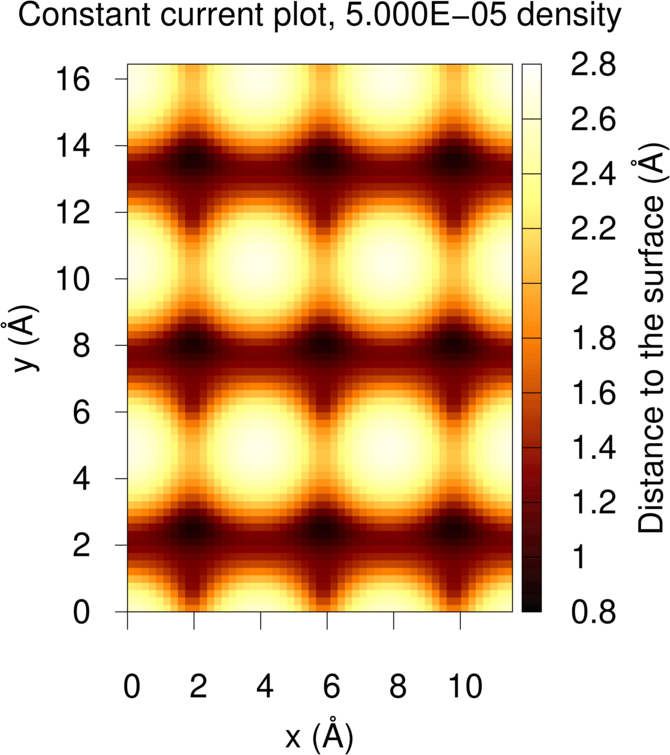
By default, the “distance to the surface” is referred to the position of the last atom before the vacuum. This reference height can be changed, if necessary, using the TOP keyword. This will only affect the scale, not the plot itself.

Constant-Height Plots

In the constant-height mode, we choose the height above the surface and the STM plot represents the LDOS, which is proportional to the current across the tip. The input is:

crystal ldos.cube
load ldos.cube
stm height 0.542 cells 3 3

In this case, we use the keyword HEIGHT. The number following HEIGHT is the height above the surface given as the fractional coordinate in the vacuum direction. If this quantity is not given, then critic2 defaults to the height of the last atom before the vacuum plus one bohr in the vacuum direction. As before, we represent a 3x3 supercell.

Running this input generates the same two files as in the constant-current case, and doing gnuplot on the .gnu file results in:

alasch

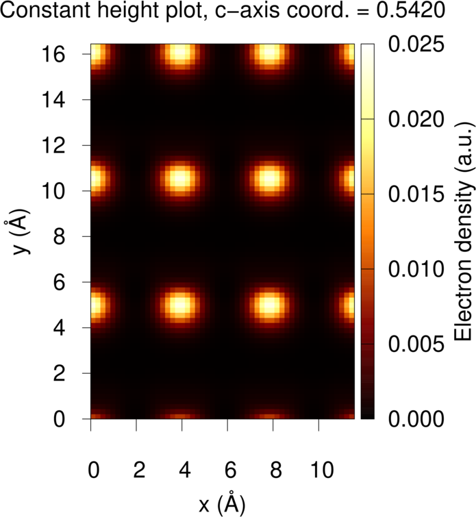
The As positioned at the corner of the unit cell is higher than the rest of the atoms, and it is shown as a bright spot in both STM plots.

Example Files Package

Files: example_14_01.tar.xz. Run the examples as follows:

QE, run the SCF and non-SCF calculations and generate the LDOS:

## generate the pseudopotentials first:
ld1.x < al.in
ld1.x < as.in
## run the SCF calculation
pw.x < alas110re.scf.in
## run the non-SCF calculation
pw.x < alas110re.nscf.in
## create the LDOS cube file
pp.x < alas110re.stm.in

Make the constant-current plot:
```
critic2 alas110re-cc.cri
gnuplot alas110re-cc_stm.gnu
```
This generates the alas110re-cc_stm.eps file containing the plot.
Make the constant-height plot:
```
critic2 alas110re-ch.cri
gnuplot alas110re-ch_stm.gnu
```
This generates the alas110re-ch_stm.eps file containing the plot.

Manual Pages

Scanning tunneling microscopy (STM) plots