Molecular Calculations

Representations of the Exchange Hole

The exchange hole can be calculated in critic2 using the xhole(id,x,y,z) chemical function. This function takes four arguments: the ID of the field (which must be a molecular wavefunction) and the coordinates of the reference point. The latter must be given in Cartesian coordinates referred to the molecular origin.

Let us assume we have the molecular wavefunction for benzene calculated using Gaussian (benzene.wfx). We load the structure and the wavefunction in critic2 using:

molecule benzene.wfx
load benzene.wfx

Because it is the first field loaded, the wavefunction field can be accessed with the $1 variable. We can, for instance, plot the exchange hole in the molecular plane:

a = 3
plane -a -a 0  a -a 0  -a a 0  101 101 field "-xhole(1,0.0,0.0,0.0)"    file xhole-0 contour lin 41 0.0 0.2
plane -a -a 0  a -a 0  -a a 0  101 101 field "-xhole(1,0.0,0.5,0.0)"    file xhole-1 contour lin 41 0.0 0.2
plane -a -a 0  a -a 0  -a a 0  101 101 field "-xhole(1,0.0,1.0,0.0)"    file xhole-2 contour lin 41 0.0 0.2
plane -a -a 0  a -a 0  -a a 0  101 101 field "-xhole(1,0.0,1.3936,0.0)" file xhole-3 contour lin 41 0.0 0.2

These four plots comprise a square from (-3,-3) to (+3,+3) angstrom with 101 points in each direction. Contour lines are represented in a linear scale from -0.2 to 0.0. The four plots have different positions for the reference point: from the center of the molecule (0,0,0) to exactly on top of a carbon atom (0,0,1.3936). The plots written by critic2 are:

xhole0 xhole1

xhole2 xhole3

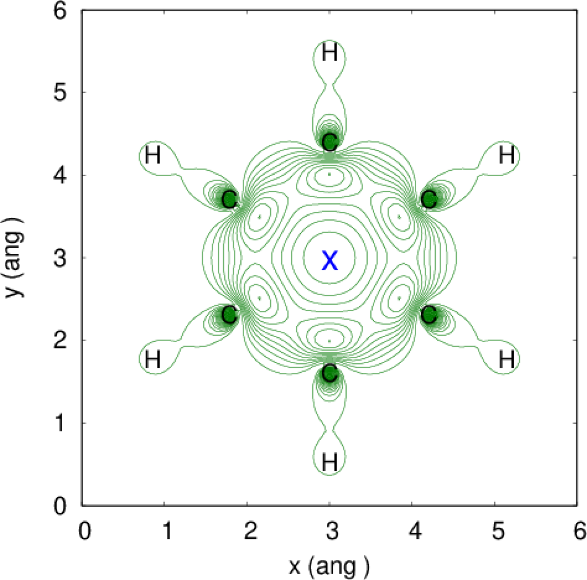
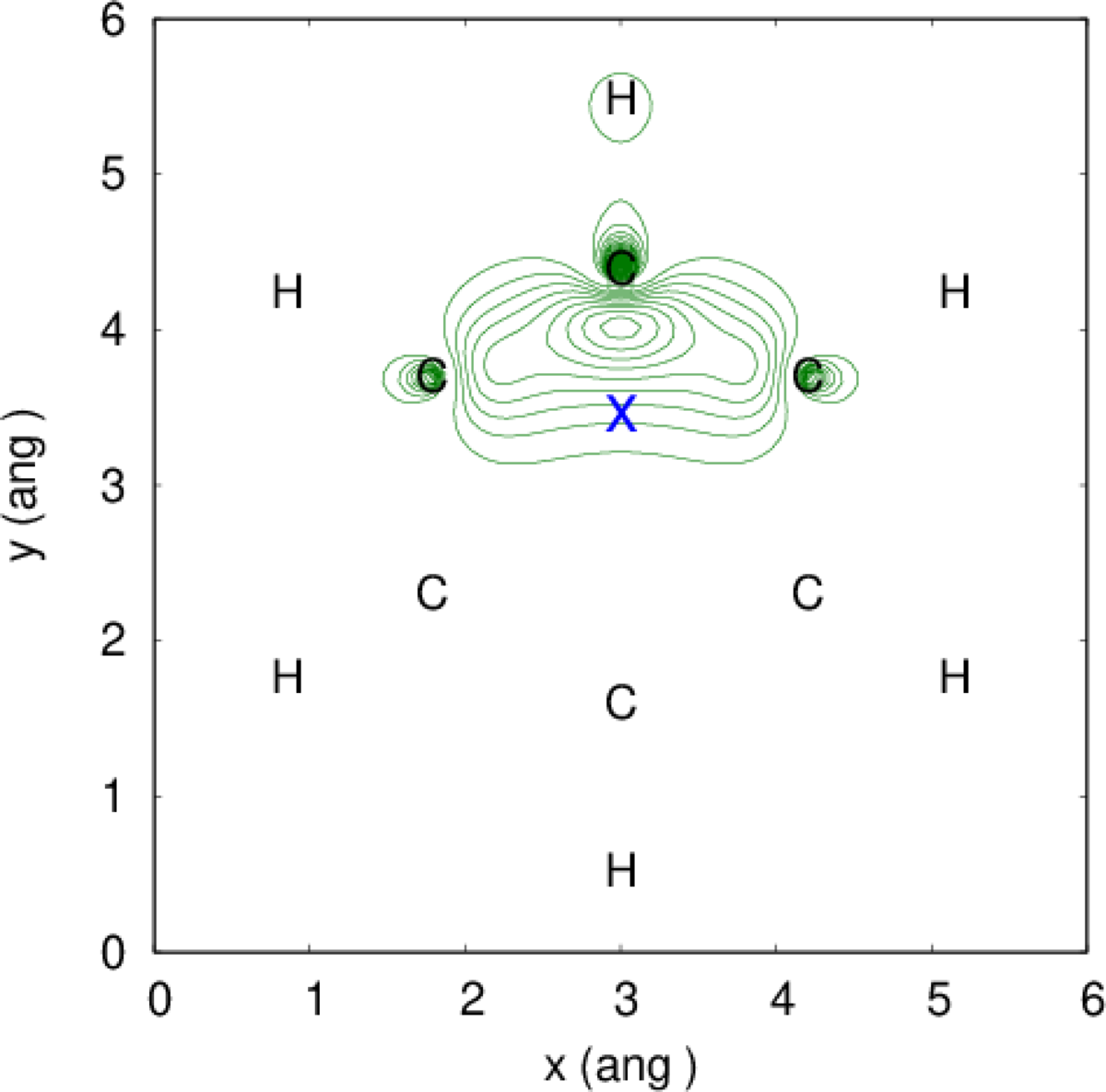
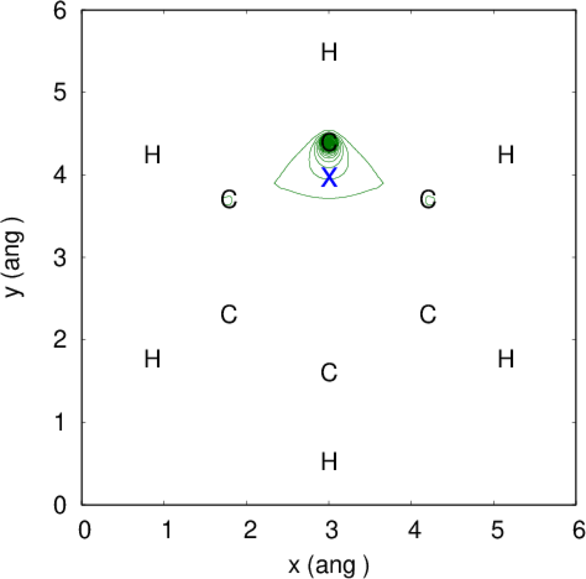
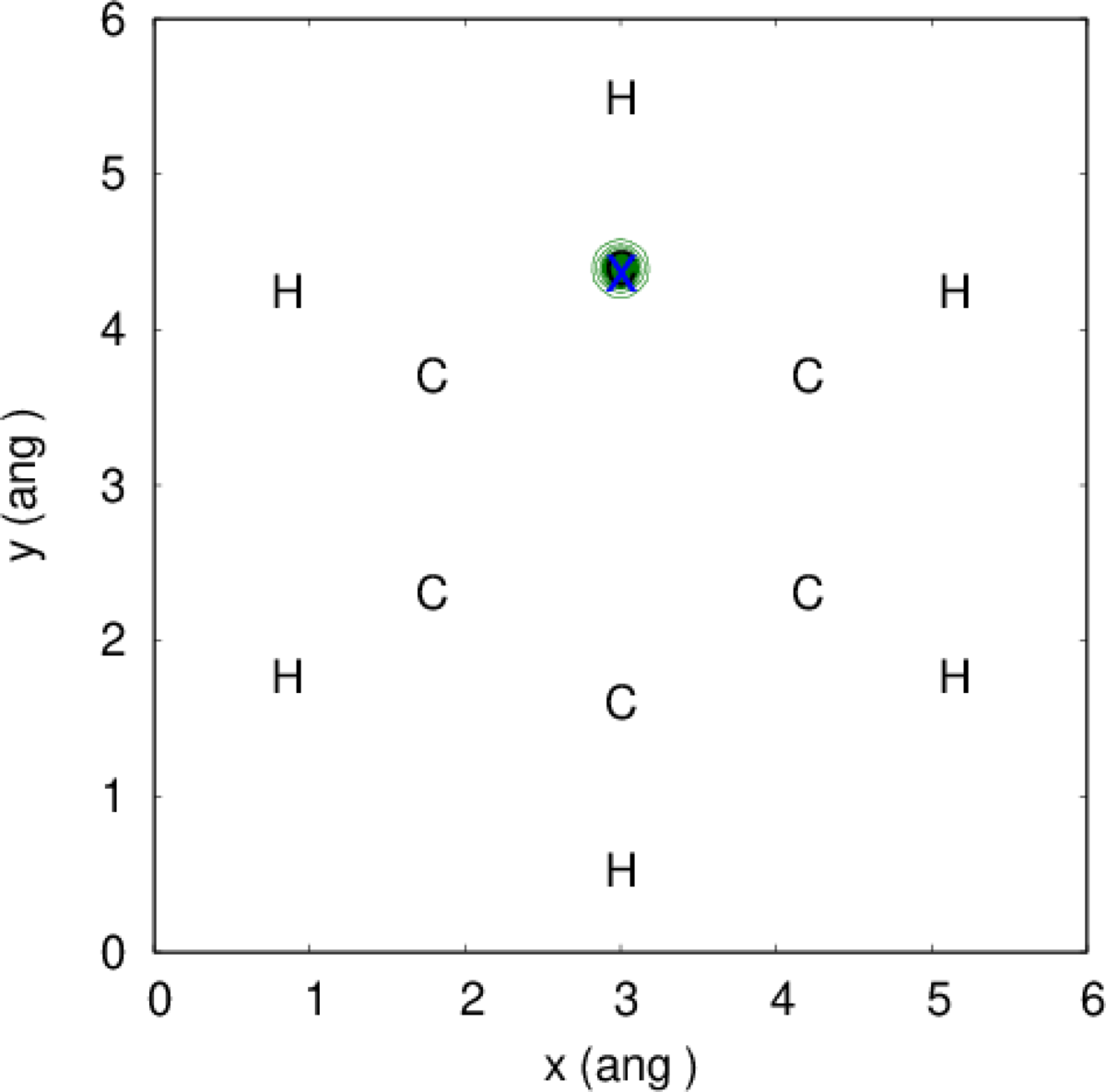
where the blue “x” indicates the reference point. The localization exchange-hole is greater when one moves the reference point closer to an atom.

We can also check the on-top depth condition for the exchange-hole, which says that the value of the exchange hole at the reference point should equal the density for the same spin:

$\begin{equation} h_x^\sigma({\bf r},{\bf r}) = -\rho_\sigma({\bf r}) \end{equation}$

This can be checked directly at any given point (for instance, (0.1,0.2,0.3)) with:

point 0.1 0.2 0.3 field "abs(xhole(1,0.1,0.2,0.3) + $1:up)"

where the exchange hole is evaluated at the reference point and compared to the up-spin density (the system is closed shell, so the up- and down-spin densities are the same). The result is:

* POINT 0.1000000  0.2000000  0.3000000
  Coordinates (ang): 0.1000000  0.2000000  0.3000000
  Expression (abs(xhole(1,0.1,0.2,0.3) + $1:up)): 1.734723476E-17

so the on-top depth of the exchange-hole at that particular point is correct. In fact, we can verify that the on-top depth of the exchange hole and the density are the same by integrating the same expression in a molecular mesh:

molcalc "abs(xhole(1,@xm,@ym,@zm) + $1:up)"

which gives:

+ Integral(abs(xhole(1,@xm,@ym,@zm) + $1:up)) = 0.00000000

Since the integrand is always positive, a zero integral means the two fields are identical. The @xm, @ym, and @zm are structural variables. They take the value of the x, y, and z coordinates of each point in the molecular mesh (in this case, in angstrom, to make them consistent with the arguments for the xhole function).

Likewise, we can verify the normalization of the exchange hole:

$\begin{equation} \int h_x^\sigma({\bf r}_1,{\bf r}_2) d{\bf r}_2= -1 \end{equation}$

with:

molcalc "xhole(1,0.0,0.0,0.0)"

which gives:

+ Integral(xhole(1,0.0,0.0,0.0)) = -1.00067590

The small deviation from the correct value (-1) comes from grid being relatively coarse.

Example Files Package

Files: example_15_01.tar.xz. Run the examples as follows:

If you can use Gaussian, run the SCF calculation and generate the wavefunction with:
```
g16 benzene.gjf
```
Older versions of Gaussian may also work. If you do not have Gaussian, a benzene.wfx wavefunction is provided in the package.
Run the critic2 input file. This file contains all the tasks in this example.
Generate the plots by running the executing the generated gnuplot scripts:
```
gnuplot xhole-0.gnu
gnuplot xhole-1.gnu
gnuplot xhole-2.gnu
gnuplot xhole-3.gnu
```
The plots are called xhole-*.eps.

Representations of the Exchange Hole

Example Files Package

Manual Pages