Locating Critical Points of Densities Given as Grids
Introduction
In critic2, the location of critical points (CPs) of the electron density and other fields is carried out by the AUTO keyword. AUTO works by applying Newton’s method repeatedly starting at a collection of starting points in the system, known as seeds. Newton requires knowledge of the first and second derivatives of the electron density. If the density is given analytically and the gradient and the Hessian can be calculated exactly, Newton’s method typically finds all critical points in the system and typically it only fails either because more seeds are required or because of the appearance of spurious critical points in the vacuum region. These two cases can be easily solved by appropriate use of the SEED and DISCARD sub-keywords of AUTO.
If the electron density is given on a grid, analytical derivatives are not available because the density is known only at a discrete set of points, the nodes of a three-dimensional uniform grid. The simplest way of trying to locate its critical points in this case is to employ three-dimensional interpolation to extend the electron density to all points in the system, and to enable the calculation of derivatives. There are two problems with this naive approach:
-
Close to the nuclei, where the density is very steep, the interpolation methods create spurious oscillations that interfere with the CP location algorithm. The oscillations are more severe in the derivatives of the electron density, and worse the higher the derivative.
-
Density grids for periodic systems (solids) are often non-orthogonal. If the grid nodes used for the interpolation depend on the grid geometry, then the result of the interpolation depends on the particular basis chosen for representing the unit cell, which introduces spuriously privileged directions in the density. This is known as lattice bias.
In a 2022 article (Otero-de-la-Roza, J. Chem. Phys. 156, 224116 (2022)) an interpolation method for the all-electron density was proposed that addresses these two problems. This method is based on polyharmonic spline interpolation combined with a smoothing function, and can be accessed by using the SMOOTHRHO option to the LOAD keyword. The number of grid nodes on which the interpolation is based (NENV) as well as the number of interpolants used in the linear combination (FDMAX) can be controlled by the user but in general touching these values is not required. Spurious critical points can still appear if the density is noisy or if the grid is not sufficiently fine.
Also, note that the SMOOTHRHO keyword is not the default interpolation method in critic2, and needs to be activated explicitly. This is because it is only suitable for interpolating all-electron densities. Other fields would require other smoothing functions (as described in the article). If you need to find critical points of other fields, please let me know.
Using VASP
The all-electron density in VASP can be obtained using the LAECHG
tag in the INCAR file. VASP writes two files, AECCAR0 and
AECCAR2, containing the core density and the reconstructed valence
electron density on the grid. The all-electron density is obtained as
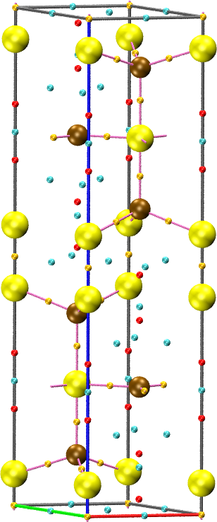
the sum of the two fields. For example, for the covellite (CuS) system
in the package:
# Read the crystal structure either of the AECCARs
crystal covellite.AECCAR0

# Calculate the reconstructed all-electron density as the sum of core
# and valence densities
load covellite.AECCAR0
load covellite.AECCAR2
load as "$1+$2" id rhoae smoothrho
reference rhoae

# Find the critical points and write them to a vmd file
auto
cpreport covellite.vmd cell border graph
(Occasionally, strange results may be obtained from the integration of
atomic charges with VASP due to noise in the AECCAR0 file. To
prevent this, do not use ADDGRID=.TRUE. in your INCAR file.)
The CPREPORT keyword is used to write the set of critical points to a vmd file for visualization, together with the graph.
Using abinit
The all-electron density can be written from a PAW calculation in
abinit using the prtden 3 keyword, but this requires the separate
calculation of the core density contributions in a
core_density_atom_type1.dat file. Instead, you can use prtden 2
and write the reconstructed valence electron density, and then employ
critic2’s core density tables to add the core contribution.
Assuming you went with prtden 2, a _PAWDEN file was generated that
contains the valence all-electron density. In a first step, we augment
this density with the core contribution and write the result to a new
grid file (rhoae.cube):
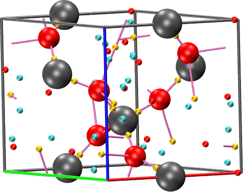
## Read the crystal structure from the PAWDEN file
crystal quartz_o_PAWDEN

## Load the reconstructed valence density and augment it with the core
## contribution. The pseudopotential charge (the number of valence
## electrons) is 4 for Si and 6 for O.
load quartz_o_PAWDEN zpsp si 4 o 6

## Write the core+valence density to a cube file (rhoae.cube). We
## cannot interpolate from the above because it is not a pure grid
## field.
cube grid field 1 file rhoae.cube
The cube file written in this way can then be used to find the CPs:
## Read the structure from the cube file.
crystal rhoae.cube

## Load the all-electron density and activate the smoothrho
## interpolation.
load rhoae.cube smoothrho

## Find the critical points and write them to a vmd file
## for visualization
auto
cpreport quartz.vmd cell border graph
Using Quantum ESPRESSO
In Quantum ESPRESSO, the reconstructed all-electron density can be
generated using a PAW calculation and the plot_num=21 option in
pp.x. This option writes a cube file (rhoae.cube) containing the
density. Finding the critical points from this cube file is
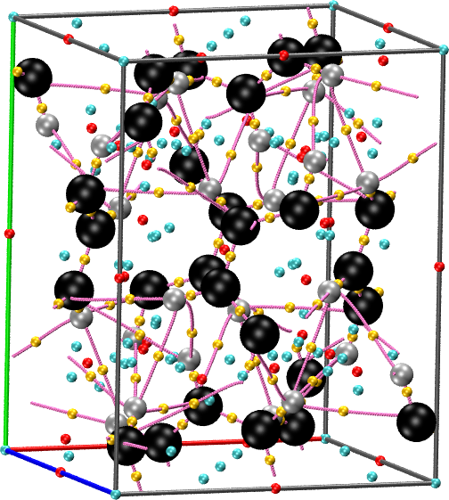
straightforward. For instance, for the benzene crystal included in the
example package:
## Read the crystal structure from the cube file
crystal rhoae.cube

## Load the density with smoothrho interpolation
load rhoae.cube smoothrho

## Find the critical points and write them to a vmd file
auto
cpreport benzene.vmd border molmotif graph
Using Molecular Cube Files (Gaussian,…)
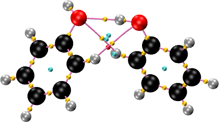
The SMOOTHRHO interpolation can be applied to any all-electron density, periodic or non-periodic. In particular, it can be used to reconstruct the density and find CPs in molecules whose electron density is given on a grid, for instance, as a cube file. The input is similar to the other examples, with two exceptions. First, the MOLECULE keyword is used to read the geometry. Second, a density cutoff is set so that critical points with very low density are discarded. This is used to prevent the appearance of spurious critical points in the vacuum region, where the density is flat and essentially zero. A value of \(10^{-5}\) atomic units is a good choice. For the phenol dimer example included in the package:
## Read the molecular geometry from the cube file.
molecule phenol_phenol.cube

## Read the electron density from the cube file and activate the
## smoothrho interpolation.
load phenol_phenol.cube smoothrho

## Locate the critical points and discard the CPs with density ($1)
## less than 1e-5 atomic units.
auto discard "$1 < 1e-5"

## Write the results to a vmd file for visualization.
cpreport phenol_phenol.vmd graph
Convergence of Critical Point Properties with Grid Size
One question that is often asked is what grid size should be used to obtain reliable properties (density, Laplacian) at the critical points, and whether these converge with the grid size. If the SMOOTHRHO interpolation method is not, it is not expected that any critical point properties, except perhaps for the density, converge with grid size. However, with SMOOTHRHO convergence happens for relatively sparse grids: It is not necessary to use massive density grids to get reliable properties.
In the qe-convergence folder, a series of QE calculations were
carried out for the benzene molecular crystal with increasing
ecutrho. The resulting grids are correspondingly larger. The
following table shows the electron density and Laplacian at the
highest-density critical point, corresponding to a carbon-carbon bond.
| ecutrho | Grid size | Density (a.u.) | Laplacian (a.u.) |
|---|---|---|---|
| 500 | (100,128,96) | 0.315384246 | -0.976211158 |
| 600 | (108,144,100) | 0.315379570 | -0.973927340 |
| 700 | (120,150,108) | 0.315369481 | -0.968755881 |
| 800 | (128,160,120) | 0.315362774 | -0.962695617 |
| 900 | (144,180,128) | 0.315375069 | -0.970508500 |
| 1000 | (144,180,128) | 0.315379333 | -0.974034357 |
| 1100 | (150,192,144) | 0.315378013 | -0.974432209 |
| 1200 | (160,200,144) | 0.315375364 | -0.970082769 |
As can be seen, even with a reasonably low ecutrho the electron density is converged to 4-5 significant digits and the Laplacian, which is much harder to calculate reliably from a grid because it involves the second derivatives, is good to 2 significant digits.
Visualization
The pictures above can be generated using vmd and the output of the CPREPORT keyword. The detailed description of how this keyword works and the visualization options is given in the manual. In short, to view the file, do:
vmd -e bleh.vmd
and you can remove the atoms by writing:
label delete Atoms all
in the Tk console.
Example Files Package
Files: example_08_01.tar.xz.