Making NCI Plots in molecules, surfaces, and solids
These examples show how to make non-covalent interaction (NCI) plots in molecules and solids. For more details on what NCI plots are, see Johnson et al.’s article and this other article for the implementation in solids, and the manual pages indicated at the end.
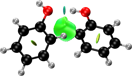
Molecules: Phenol Dimer
NCI plots can be generated in two ways. If you have the structure and the self-consistent electron density, you can calculate the NCI domains using them. Otherwise, the promolecular density can be used for the generation of the NCI domains, in which case only the structure is required.
A simple NCI plot input file for phenol dimer using the promolecular density is:
molecule phenol_phenol.xyz 0

nciplot
endnciplot
First, the molecular structure of the phenol dimer (contained in an
xyz file) is loaded into critic2 with the
MOLECULE keyword. Then, the
NCI plot is generated by calling the nciplot/endnciplot
environment. A number of optional keywords
can be used in this environment to tune the behavior of
NCIPLOT, a few of which are described in this example. Please consult
the NCIPLOT keyword entry in the manual
for details.
The 0 after the MOLECULE command instructs critic2 to restrict the
molecular cell to the smallest box that encompasses the molecular
structure (i.e. a box with zero border). The same effect can be
achieved using the MOLCELL
keyword:
molcell 0
after loading the structure with MOLECULE. The molecular cell determines the size of the grid in which the NCI plot quantities (density, reduced density gradients, etc.) will be calculated. A small molecular cell has the double advantage of making the calculation cheaper (because you need smaller grids) and also of restricting the NCI plot to the region of interest. The only downside is that one of your NCI domains may be cut off, in which case you will have to increase this number somewhat.
Running the example above generates a number of files. You can view the results using the vmd program. To open the file, use:
vmd -e phenol_phenol.vmd
Rotate the molecule into the position you want and do File -> Render -> Tachyon (internal, in memory) and press “Start rendering”. This will generate the NCI plot file.
In general, it is better if you have run the calculation and have the
self-consistent density for the system from which to make the NCI
plot. This density can be read in any format understood by
critic2. In this example, we can use a
wfx wavefunction file from Gaussian:
molecule phenol_phenol.wfx 0
load phenol_phenol.wfx
nciplot
endnciplot
Note the only difference is that the structure and density are both read from the wavefunction file, and therefore used in the NCI plot.
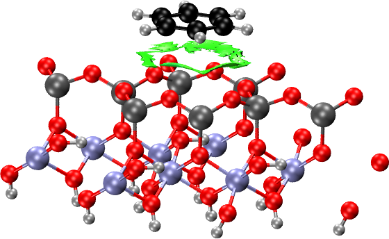
Surfaces: Benzene on Kaolinite
Now we consider making the NCI plots of a molecule (benzene) on an
inorganic surface, kaolinite (001). The equilibrium structure was
calculated using Quantum ESPRESSO in two cases: when the benzene
molecule is adsorbed to the hydrophobic side (hb) and when it is
adsorbed to the hydrophilic side (hl). The structure and
self-consistent electron densities are contained in the
hbpar1_rho.cube and hlpar1_rho.cube cube files, respectively,
generated using QE’s pp.x program.
We consider absorption to the hydrophobic surface first
(hbpar1_rho.cube). We could use an NCIplot input file identical to
the one in the previous section for molecular systems. However, in
surfaces and solids, there are typically too many NCI domains and it
is often the case that we want to focus on a particular interaction.
In this case, we want only the NCI domains that arise from the
interaction between the molecule and the surface. To focus only on
these interactions, we create .xyz files containing the relevant
fragments (one for benzene and another for the surface) and then pass
those to the NCIPLOT environment. That way, only the domains that
involve interactions between the two fragments will be plotted.
Therefore, we first need to write the structure contained in the cube files and select the fragments for the NCIplot calculation. To do this, we first write an xyz file containing the surface and the molecule:
crystal hbpar1_rho.cube
write cell.xyz border 1 1 2
This creates an xyz file (cell.xyz) containing the slab plus the
molecule. The 1 1 2 instructs critic2 to write a 1x1x2 supercell of
the original system, so that a whole slab is contained in the
file. The BORDER keyword makes all atoms at the border of the
supercell be included in the file. You can now open this file with
your favorite program (I use avogadro) and cut away from it the
benzene and the surface underneath, and save the two systems to
separate xyz files (hbpar1_benzene.xyz and hbpar1_surface.xyz).
Lastly, we generate the NCI plot with the input file:
crystal hbpar1_rho.cube
load hbpar1_rho.cube
nciplot
  fragment hbpar1_benzene.xyz
  fragment hbpar1_surface.xyz
  nstep 100 100 100
endnciplot
We first load the surface structure from the cube file, then the self-consistent electron density, which becomes the reference field and therefore will be used by NCIPLOT to generate the NCI domains. The xyz files containing the fragments written in the previous step are passed to the NCIPLOT environment, which ensures that only the NCI domains contained between those fragments are plotted. Lastly, the default grid used for the NCI plots (0.1 bohr between points in each direction) is too large for this example. Therefore, we use the NSTEP option to limit the grids used for the plot to 100 points in each direction. In a production calculation, you should use a finer grid (perhaps the default grid) to improve the quality of the plot and avoid artifacts.
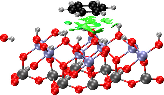
For the case of benzene on the hydrophilic surface, the procedure to make the NCI plots is entirely analogous. First, we create an xyz file containing the surface:
crystal hlpar1_rho.cube
write cell.xyz border 1 1 2
Then, we cut the benzene and surface fragments into their respective
xyz files (hlpar1_benzene.xyz and hlpar1_surface.xyz) and finally
we generate the NCI plot with:
crystal hlpar1_rho.cube
load hlpar1_rho.cube
nciplot
  fragment hlpar1_benzene.xyz
  fragment hlpar1_surface.xyz
  nstep 100 100 100
endnciplot
As in the molecular case, the promolecular density can be used instead of the calculated electron density if the latter is not available. To do this, simply remove the LOAD command. This requires only the surface structure.
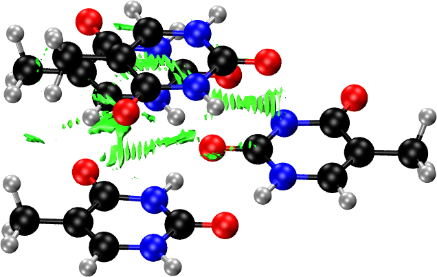
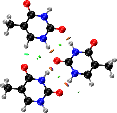
Solids: Thymine Molecular Crystal
Same as in the surface case, NCI plots of a periodic crystal are very busy because of the large number of NCI domains and atoms. We need to use the FRAGMENT keyword to focus the NCI plot on the interactions we are interested in. In this example we examine the thymine crystal, in which there are two dominant interactions: the intra-layer hydrogen bonds and the inter-layer stacking interactions.
Before calculating the NCI plots, we need to generate the fragment
structures. The equilibrium structure and electron density were
calculated with Quantum ESPRESSO, and both are contained in the
thymine_rho.cube file. To create the fragments, we use the following
input:
crystal thymine_rho.cube
write cell.xyz molmotif
This creates an xyz file (cell.xyz) containing the atoms in the unit
cell. The MOLMOTIF option makes critic2 include all atoms from
neighboring cells necessary to complete all molecular structures. If a
larger unit cell is needed to define the fragments, we could do:
crystal thymine_rho.cube
write cell.xyz molmotif 2 2 2
to perform the same operation on a 2x2x2 supercell. You can also write all the monomers in the unit cell with:
write thymine_monomers.xyz molmotif nmer 1
and all the dimers with:
write thymine_pairs.xyz molmotif nmer 2
Using avogadro, we now cut the fragments of interest. To examine the
intra-layer hydrogen bond, we select three adjacent molecules
interacting via hydrogen bonds within the same layer
(thymine_intra*.xyz). For the stacked layer interaction, we pick a
three-molecule motif from one layer (thymine_inter1.xyz) and a
single molecule, exactly above this triangular motif, from an adjacent
layer (thymine_inter1.xyz).
Now we generate the NCI plot for the inter-layer stacking interaction with:
crystal thymine_rho.cube
load thymine_rho.cube

nciplot
 fragment thymine_inter1.xyz
 fragment thymine_inter2.xyz
 nstep 100 100 100
endnciplot
The two fragments we generated before (the triangular motif and the single molecule on top of it) are passed to the NCIPLOT environment using the FRAGMENT option. This restricts the NCI domain to only those that appear between the selected fragments. The NSTEP option reduces the number of points in the calculated density and reduced density gradient grids. For production calculations, you should use the defaults (remove the NSTEP) or increase these numbers; otherwise oscillations appear, as shown in the NCI plots below.
For the intra-layer interactions, we pass to the FRAGMENT option the three fragments corresponding to the three hydrogen-bonded molecules within the same layer:
crystal thymine_rho.cube
load thymine_rho.cube

nciplot
 fragment thymine_intra1.xyz
 fragment thymine_intra2.xyz
 fragment thymine_intra3.xyz
 nstep 175 175 75
endnciplot
As before, we use NSTEP to restrict the number of points in the calculated grids. You should use the defaults, or at least a finer grid, for production plots.
As before, the promolecular density can be used instead of the calculated electron density if the latter is not available. To do this, simply remove the LOAD commands. In this case, only the structure of the molecular solid is needed.
Example Files Package
Files: example_12_01.tar.xz.